Elasticity of Supply: Percentage and Geometric Methods

A pottery studio gets a chance to sell its cups at a higher price. The owner would love to make more. But can the kiln hold another batch? Is there enough clay? Can another potter join this week?

The higher price creates an incentive. The studio’s ability to respond determines how much extra it supplies.

Price elasticity of supply measures that response in percentage terms. Once you understand this, the numerical formula and the graph become two ways of asking the same question: how responsive is quantity supplied to a change in the good’s own price?

What Does Elasticity of Supply Measure?

Price elasticity of supply, written as Es, is the percentage change in quantity supplied divided by the percentage change in price, with other supply conditions held constant. It measures a movement along a supply curve, rather than a shift caused by new technology or changing input prices. NCERT: The Theory of the Firm under Perfect Competition

In our studio example, compare cups supplied per week before and after the price change. Do not compare a daily quantity with a monthly quantity.

Suppose a 10% price rise leads to:

• A 25% quantity increase: Es = 25 / 10 = 2.5.
• A 10% quantity increase: Es = 10 / 10 = 1.
• A 4% quantity increase: Es = 4 / 10 = 0.4.

All three studios supply more. Their responsiveness differs.

If movement and shift still feel similar, first revisit supply schedules, curves, and shifts.

Choose the Method From the Information Given

What the question gives you	Your approach	What to watch
Percentage changes in price and quantity	Divide quantity percentage by price percentage	Keep the order correct
Old and new price and quantity; original-value percentage method requested	Use the old price and old quantity as bases	Do not mix old and new bases
Two observations; midpoint or arc method requested	Use average price and average quantity as bases	This can give a different number
A point on a straight supply line	Use the geometric intercept rule	Extend the line to the quantity axis
A smooth curved supply line	Use a tangent at the specified point	The curve’s distant intercept is not enough

If the method is unspecified, follow the convention taught for that exercise and state your choice. The original-value percentage method is used for the main numericals below; the midpoint method has its own section.

Percentage Method: The Formula You Can Rebuild

Let P0 and Q0 be the original price and quantity, and P1 and Q1 be the new values.

Percentage change in quantity = [(Q1 - Q0) / Q0] x 100

Percentage change in price = [(P1 - P0) / P0] x 100

Divide the first by the second. The two factors of 100 cancel, giving:

Es = [(Q1 - Q0) / (P1 - P0)] x (P0 / Q0)

This is also written as Es = (change in Q / change in P) x (original P / original Q).

The original price and quantity must be nonzero for these percentage bases to work, and the observed price change must be nonzero to calculate this ratio directly.

Example 1: A Price Rise and an Elastic Response

A studio supplies 240 cups a week at Rs 80 each. At Rs 100, it supplies 330 cups. Other supply conditions remain unchanged.

First, separate levels from changes:

Item	Price	Weekly quantity
Original value	Rs 80	240 cups
New value	Rs 100	330 cups
Change	Rs 20	90 cups

Quantity change = (90 / 240) x 100 = 37.5%.

Price change = (20 / 80) x 100 = 25%.

Es = 37.5 / 25 = 1.5.

Supply is elastic over this change using the original-value method: quantity rises proportionately more than price.

Check with the shorter formula:

Es = (90 / 20) x (80 / 240) = 1.5.

Notice that the answer is 1.5, not 1.5%, Rs 1.5, or 1.5 cups. Dividing one percentage by another leaves a number without units.

Example 2: Falling Price Does Not Automatically Mean Negative Elasticity

A supplier reduces its weekly quantity from 500 to 440 units when price falls from Rs 50 to Rs 40.

Change in Q = 440 - 500 = -60.

Change in P = 40 - 50 = -10.

Es = (-60 / -10) x (50 / 500) = 0.6.

Equivalently, quantity falls by 12% and price falls by 20%, so Es = (-12) / (-20) = 0.6. The two negative signs cancel. Supply is inelastic.

Example 3: Find the Missing Quantity

At Rs 40, a firm supplies 600 units. Price rises to Rs 44. Its elasticity for this change, measured on original values, is 1.25. Find the new quantity.

Price increase = (4 / 40) x 100 = 10%.

Percentage quantity increase = Es x percentage price increase.

So quantity increases by 1.25 x 10% = 12.5%.

Extra quantity = 12.5% of 600 = 75 units.

New quantity = 600 + 75 = 675 units.

The question asks for the new level, so stopping at 75 would leave the answer incomplete. If an elasticity were given only at one point on a curved supply function, using it for a finite price change would generally be an approximation instead.

Example 4: Recover Quantity From Total Revenue

A numerical sometimes gives revenue instead of quantity. Suppose all units supplied are sold. At Rs 30 each, total revenue is Rs 9,000. At Rs 36, total revenue becomes Rs 12,960.

Use quantity = total revenue / price first:

• Q0 = 9,000 / 30 = 300 units.
• Q1 = 12,960 / 36 = 360 units.

Es = (60 / 6) x (30 / 300) = 1.

Revenue rose by 44%, but quantity rose by only 20%. Revenue includes both the price effect and the quantity effect, so its percentage change cannot replace the quantity change in the elasticity formula.

Read the Five Degrees of Supply Elasticity

Value of Es	Description	Meaning
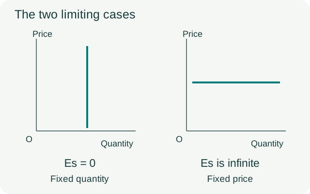
0	Perfectly inelastic	Quantity remains fixed as price changes
Between 0 and 1	Relatively inelastic	Quantity changes by a smaller percentage than price
1	Unit elastic	Quantity and price change by equal percentages
Greater than 1, but finite	Relatively elastic	Quantity changes by a larger percentage than price
Infinite	Perfectly elastic	The idealized supply curve is horizontal

A vertical supply line shows fixed quantity. A horizontal supply line is the limiting case of infinite responsiveness at a given price; it does not mean zero elasticity merely because price is unchanged. These are idealized polar cases. OpenStax: Polar Cases of Elasticity and Constant Elasticity

Geometric Method: One Ratio, Three Cases

For an upward-sloping straight supply line, choose a point A with positive price and quantity. Drop a perpendicular from A to the quantity axis at B. Call the origin O. Extend the supply line, if necessary, until it meets the quantity axis at T.

Then Es at A = TB / OB, using horizontal segment lengths. This produces three cases: T left of O gives Es greater than 1; T at O gives Es equal to 1; T between O and B gives Es less than 1. NCERT: Geometric Method, section 4.7

Why Does TB / OB Work?

You do not need to memorize an unexplained picture. In triangle TBA:

• Vertical height AB represents the price at A.
• Horizontal distance TB is the run of the straight line from its quantity-axis intercept.
• Therefore, change in Q / change in P along this line equals TB / AB.
• At A, P / Q equals AB / OB.

Multiply: Es = (TB / AB) x (AB / OB) = TB / OB.

The heights cancel. That is why the final calculation uses two horizontal distances, not the sloping length TA.

Case 1: The Supply Line Cuts the Positive Price Axis

Take the line Q = 4P - 80. At P = 40, Q = 80.

At Q = 0, P = 20, so the economically relevant rising line starts on the price axis above the origin. Extending the same line backwards to P = 0 gives Q = -80.

Thus T lies 80 quantity units to the left of O. At our chosen point, B lies 80 units to the right of O.

TB = 80 + 80 = 160.

OB = 80.

Es = 160 / 80 = 2, which is greater than 1.

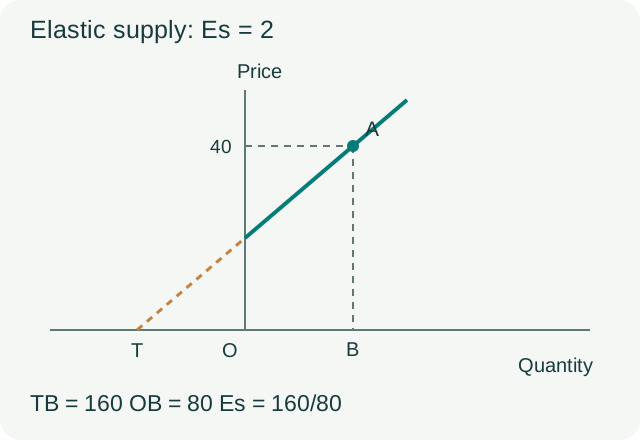
The negative quantity is a geometric extension used for measuring the line. It does not mean the firm actually supplies negative cups.

Case 2: The Supply Line Passes Through the Origin

Take Q = 2P. At P = 40, Q = 80. Setting P = 0 gives Q = 0, so T and O coincide.

TB = OB = 80.

Es = 80 / 80 = 1.

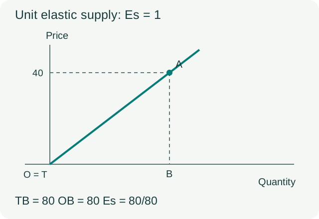
Try P = 60: Q becomes 120. Both have increased by 50%. Try a different line, Q = 10P: a 50% price rise still produces a 50% quantity rise.

Therefore, every positively sloped straight supply line through the origin is unit elastic at its positive-price, positive-quantity points. It need not make a 45-degree angle. At the origin itself, the usual percentage formula has zero bases and is not defined.

Case 3: The Supply Line Cuts the Positive Quantity Axis

Take Q = 40 + 2P. At P = 40, Q = 120. Setting P = 0 gives Q = 40, so T is to the right of O.

TB = 120 - 40 = 80.

OB = 120.

Es = 80 / 120 = 2/3, or approximately 0.67.

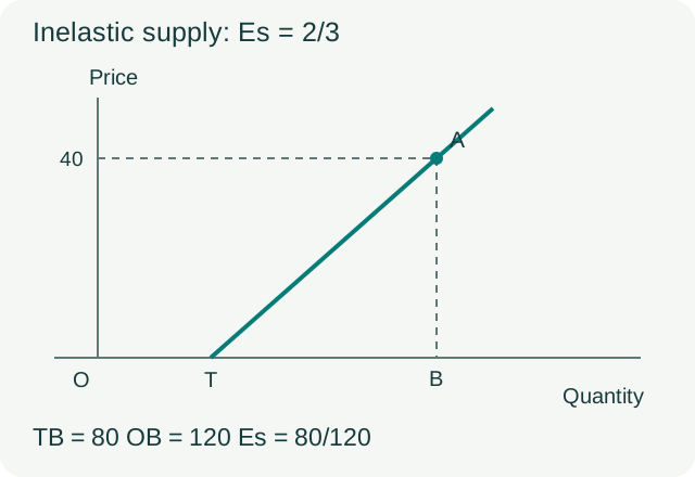
Do not calculate 40 / 120. That would use OT, whereas the numerator needs the distance from T to B.

Check the Diagrams With the Percentage Method

Raise price from Rs 40 to Rs 50 in each of the three original examples. This is a 25% increase.

Supply equation	Q at P = 40	Q at P = 50	Quantity increase	Es on original values
Q = 4P - 80	80	120	50%	2
Q = 2P	80	100	25%	1
Q = 40 + 2P	120	140	16.67% approximately	0.67 approximately

The numerical answers match the geometric answers at the starting points. This works exactly here because each supply function is linear: change in Q / change in P is constant along each line.

On a curved supply function, a ratio calculated from two separated observations describes a finite change. Point elasticity instead uses the slope of the tangent at one point.

Why Slope Alone Can Mislead You

Compare two of our equations at P = 40:

• Q = 2P gives Q = 80 and Es = 1.
• Q = 40 + 2P gives Q = 120 and Es = 2/3.

Both have change in Q / change in P equal to 2. With price on the vertical axis, both have slope change in P / change in Q equal to 1/2. Yet their elasticities differ because their P / Q ratios differ.

For the second equation, move to P = 80. Now Q = 200 and Es = 2 x (80 / 200) = 0.8. The line has the same slope, but its elasticity has changed from about 0.67 to 0.8.

For a smooth curve, draw the tangent at A and use the tangent’s quantity-axis intercept as T. The same triangle calculation measures the local response. Do not extend a chord joining two distant points and call it the tangent.

Original-Value Method vs Midpoint Method

Return to the pottery example: price rises from Rs 80 to Rs 100 and quantity rises from 240 to 330. We obtained Es = 1.5 using original values.

The midpoint method divides each change by the average of its two endpoint values. Its advantage is that reversing the direction between the same two observations leaves the elasticity unchanged. OpenStax: Price Elasticity of Demand and Price Elasticity of Supply

Average Q = (240 + 330) / 2 = 285.

Average P = (80 + 100) / 2 = 90.

Midpoint Es = (90 / 20) x (90 / 285) = 27/19, or approximately 1.42.

If we reverse the movement and use original values again, the starting point is now P = 100 and Q = 330:

Es = (-90 / -20) x (100 / 330) = 15/11, or approximately 1.36.

These results use different percentage bases. There is no arithmetic contradiction.

What Makes a Producer More Responsive?

Go back to the pottery studio. Imagine the same price opportunity under four different conditions:

1. An unused kiln is available. Another batch can be fired without waiting for new equipment. Spare capacity makes expansion easier.
2. Finished cups are in storage. Some extra supply can come from stock, so current sales need not wait for new production.
3. Special clay is difficult to obtain. The owner cannot respond much if an essential input is unavailable.
4. The higher price lasts for a year. There may be time to train staff or add equipment, allowing a larger response than in one afternoon.

Time and production constraints help explain why supply is often more responsive over longer periods. They do not guarantee infinite elasticity. For example, even a year may be too short to obtain a scarce site or train a specialist. NIOS: Price Elasticity of Supply, lesson 20

For a short explanation question, connect the factor to a specific bottleneck. “More time means more elastic supply” is less helpful than explaining what the producer can change with that time.

Mistakes to Catch Before You Submit

• Using change in price / change in quantity: elasticity needs the quantity response divided by the price change, then the correct base ratio.
• Using Q1 as one base and P0 as the other: both bases must belong to the same method.
• Confusing an extra 75 units with a new total of 75: add or subtract the change from the original quantity.
• Measuring the diagonal of the supply line: the geometric numerator and denominator are horizontal lengths.
• Calling every upward line elastic: an upward line can have Es below, equal to, or above 1.
• Treating a supply shift as an own-price response: a cheaper input changes supply conditions; it is not simply movement along the old curve.
• Writing units after Es: give units for price and quantity, but not for the elasticity coefficient.

Practice: Try These Before Reading the Answers

Use original values unless the question explicitly asks for the midpoint method.

1. Price rises from Rs 25 to Rs 30; quantity rises from 400 to 520 units. Find Es and classify supply.
2. Price falls from Rs 80 to Rs 72; quantity falls from 250 to 240 units. Find Es.
3. Es is 0.8 for a 15% price increase. Original quantity is 500 units. Find the new quantity.
4. At A, OB = 100 quantity units. T is 30 units to the left of O. Find Es geometrically.
5. At A, OB = 150. T is 50 units to the right of O, between O and B. Find Es.
6. A straight supply line through the origin looks very steep. What is Es at its positive-price points?
7. For Q = 30 + 3P, calculate point elasticity at P = 20.
8. Price rises from Rs 20 to Rs 30 and quantity rises from 100 to 160. Calculate midpoint Es.

Answers With Working

1. Quantity rises by 30%; price rises by 20%. Es = 1.5, elastic.
2. Quantity falls by 4%; price falls by 10%. Es = 0.4, inelastic.
3. Quantity rises by 0.8 x 15% = 12%. Extra quantity is 60, so new quantity = 560 units.
4. TB = 30 + 100 = 130. Es = 130 / 100 = 1.3.
5. TB = 150 - 50 = 100. Es = 100 / 150 = 2/3, approximately 0.67.
6. Es = 1. The line passes through the origin; its visual steepness does not change this result.
7. Q = 30 + 3(20) = 90. Es = 3 x (20 / 90) = 2/3. Alternatively, TB = 90 - 30 = 60 and OB = 90.
8. Average Q = 130; average P = 25. Es = (60 / 10) x (25 / 130) = 15/13, approximately 1.15.

Frequently Asked Questions

What is the formula for price elasticity of supply?

Es equals the percentage change in quantity supplied divided by the percentage change in price. With original values, use Es = (change in Q / change in P) x (original P / original Q).

What is the difference between the percentage and geometric methods?

The percentage method uses changes in numerical values. The geometric method uses the line or tangent at a specified point and measures TB / OB, where T is its quantity-axis intercept and B is directly below the point.

Does a straight supply curve always have constant elasticity?

No. Our line Q = 40 + 2P gives Es of about 0.67 at P = 40 and 0.8 at P = 80. A positively sloped straight line through the origin is the special case with Es = 1 throughout its positive-price portion.

Why is a supply line through the origin unit elastic?

Its price and quantity are proportional. Doubling price doubles quantity, for example. Geometrically, T coincides with O, so TB and OB are equal.

What if the supply line meets the price axis above the origin?

Extend it backwards to the quantity axis. Its intercept T will be left of O. Then TB exceeds OB, so elasticity is greater than 1 at positive-price, positive-quantity points.

Does a positive quantity-axis intercept mean inelastic supply?

For an upward-sloping straight supply line, yes, at positive-price points. T lies between O and B, so TB / OB is less than 1. Use the tangent’s intercept instead if the supply curve is curved.

Can I use the demand elasticity lower-segment rule for supply?

Do not transfer that rule to a supply diagram. For the supply construction used here, identify the quantity-axis intercept and calculate the horizontal ratio TB / OB.

Why do I get different answers using original values and midpoint values?

The percentage bases differ. The midpoint method uses averages, while the original-value method uses the starting values. State and follow the method required by the question.

Is supply elasticity negative when price falls?

For an ordinary upward-sloping supply curve, both price and quantity supplied fall together. Their percentage changes are both negative, so their ratio is positive. Check the actual relationship rather than assuming the sign from price alone.

Is supply always perfectly elastic in the long run?

No. More time often allows a stronger response, but capacity, scarce inputs, land, skills, and rising costs can still restrict expansion. Longer-run flexibility does not automatically imply a horizontal supply curve.