Linear Programming Graphs: Feasible Regions and Corner Points

You have drawn all the lines. Several points look like corners. Now comes the part that makes you hesitate: which area should you shade, and which points belong in the answer table?

In linear programming, the graph answers two separate questions. First, which choices are allowed? Then, among those choices, which gives the best result?

Picture a garden whose shape is defined by several fences. A place inside one fence might still be outside another. The usable garden is the space that satisfies every boundary together. Your feasible region works in exactly that way.

This guide walks through the graphical method with original examples, labelled diagrams, and a few checks you can use when a graph feels confusing. We will also tackle unbounded regions, equal optimal values, and intersections that look convincing but fail a constraint.

What are the feasible region and the objective function?

Suppose a workshop makes two products. Let x and y represent the quantities produced.

Restrictions such as x + y <= 9 describe what the workshop can manage. These are constraints. An expression such as P = 50x + 40y measures total profit. This is the objective function, which the question asks you to maximise or minimise. OpenStax introduces these roles in its linear programming lesson.

Three terms will keep appearing:

Term	What it means
Feasible point	A pair (x, y) satisfying every constraint
Feasible region	All the feasible points taken together
Optimal solution	A feasible point giving the required best value

A feasible solution is allowed, but it need not be the best. Also, the solution point and the objective value are different things. If a problem gives (x, y) = (5, 4) and profit Rs 410, a complete answer states both.

Throughout the worked examples, <= means less than or equal to, and >= means greater than or equal to. Unless we explicitly discuss whole-number restrictions, the variables can take any real values satisfying the constraints.

How to shade a linear inequality

Take x + 2y <= 8.

Replace the inequality temporarily with the boundary equation x + 2y = 8. Two convenient points are (8, 0) and (0, 4). Join them with a straight line.

Now test a point away from that line. The origin is convenient:

At (0, 0):
x + 2y = 0
0 <= 8 is true.

The required side contains the origin. Since equality is allowed, the boundary line belongs to the solution too.

For x + 2y >= 8, draw the same line. This time the origin fails, so choose the opposite side. OpenStax’s section on systems of inequalities explains the test-point and common-overlap method.

Do not memorise “less than means below”

The coefficient of y matters. Consider:

x - 2y >= 4
-2y >= 4 - x
y <= (x - 4)/2

Dividing by a negative number reverses the inequality. Although the original sign is >=, the required side is below this line.

A direct check agrees. (6, 0) gives 6 >= 4, which is true. (0, 3) gives -6 >= 4, which is false. Substitution is safer than guessing from the original sign.

What if the line passes through the origin?

For 2x - y <= 0, the origin lies on the boundary. It cannot tell you which side to choose because it gives equality.

Use (0, 1) instead. It gives -1 <= 0, so the side containing (0, 1) is allowed. Equivalently, rearranging gives y >= 2x.

Remember vertical lines, horizontal lines, and the axes

Constraint	Region to keep
x <= 6	Left of x = 6, including the line
x >= 2	Right of x = 2, including the line
y <= 4	Below y = 4, including the line
y >= 3	Above y = 3, including the line
x >= 0, y >= 0	First quadrant, including its axes

When a constraint has a strict sign, < or >, its boundary is excluded and is drawn dashed. Ordinary school linear programming examples usually include their boundaries. Do not silently replace a strict sign with a non-strict one.

How several shaded regions become one feasible region

Every constraint is an additional condition. You need their intersection, meaning the common overlap, rather than the combined area covered by any one inequality.

For a paper graph, draw the boundary lines clearly and mark the allowed side of each with a small arrow. Once you see the shared area, shade that final region neatly. This keeps the drawing readable when three or more constraints overlap.

A valid region may be enclosed, may extend indefinitely, or may be empty. It can even shrink to a segment or a single point. Two separate shaded islands are a warning sign for an ordinary linear programming problem: its feasible set is convex, so the segment joining any two feasible points remains feasible. MIT’s geometry lecture explains this property.

Worked example 1: maximise profit with three constraints

A small workshop makes desk trays and pen stands. It earns Rs 50 per tray and Rs 40 per stand. Assume everything produced is sold.

Let x be the number of trays and y the number of stands made per day.

The workshop has these limits:

• It can pack at most 9 items: x + y <= 9.
• A tray uses 2 cutting slots and a stand uses 1, with 14 available: 2x + y <= 14.
• A tray uses 1 finishing slot and a stand uses 3, with 21 available: x + 3y <= 21.
• Production cannot be negative: x >= 0, y >= 0.

The objective is to maximise P = 50x + 40y.

Step 1: plot the boundary lines

Boundary	On the x-axis	On the y-axis
x + y = 9	(9, 0)	(0, 9)
2x + y = 14	(7, 0)	(0, 14)
x + 3y = 21	(21, 0)	(0, 7)

You do not need to squeeze the intercept (21, 0) onto a small graph. For that line, you could plot (0, 7) and (3, 6). Similarly, (5, 4) and (7, 0) give two visible points on 2x + y = 14.

Use a clearly stated, consistent scale on each axis. Exact intersection coordinates will come from algebra, so you do not have to estimate them from thick pencil lines.

Step 2: keep the common overlap

The origin satisfies all three resource inequalities. Keep the origin side of each line, within the first quadrant.

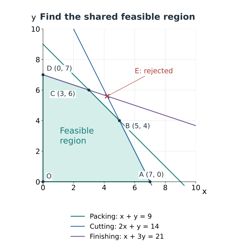
Following the boundary around the shaded region gives O, A, B, C, D.

Step 3: calculate the corners exactly

At the origin, O = (0, 0).

On the x-axis, set y = 0. The restrictions become x <= 9, x <= 7, and x <= 21. The tightest is x <= 7, giving A = (7, 0).

At B, solve the packing and cutting boundaries:

x + y = 9
2x + y = 14

Subtract the first equation from the second:
x = 5
Then y = 9 - 5 = 4.

B = (5, 4)

Check the remaining resource constraint: 5 + 3(4) = 17 <= 21. B is feasible.

At C, solve the packing and finishing boundaries:

x + y = 9
x + 3y = 21

Subtract the first equation from the second:
2y = 12, so y = 6.
Then x = 9 - 6 = 3.

C = (3, 6)

The cutting check gives 2(3) + 6 = 12 <= 14. C is feasible too.

On the y-axis, set x = 0. The restrictions are y <= 9, y <= 14, and y <= 7. Therefore, D = (0, 7).

Step 4: reject the tempting extra intersection

The cutting and finishing lines also cross:

2x + y = 14
x + 3y = 21

y = 14 - 2x
x + 3(14 - 2x) = 21
-5x = -21
x = 21/5 = 4.2

y = 28/5 = 5.6

But x + y = 9.8, which exceeds the packing limit of 9. So E = (4.2, 5.6) must be rejected.

If you evaluate profit there, you get Rs 434. That attractive number is irrelevant because the workshop cannot produce that combination under its packing limit.

This is the difference between an intersection of drawn lines and a vertex of the feasible region. James Jones’s Richland College lesson also highlights this distinction.

Step 5: test the valid corner points

Corner	Calculation of 50x + 40y	Profit
O (0, 0)	0 + 0	Rs 0
A (7, 0)	350 + 0	Rs 350
B (5, 4)	250 + 160	Rs 410
C (3, 6)	150 + 240	Rs 390
D (0, 7)	0 + 280	Rs 280

The workshop should make 5 trays and 4 stands, giving a maximum daily profit of Rs 410 under these assumptions.

At this point, all 9 packing places and all 14 cutting slots are used. Finishing uses 17 of its 21 slots, leaving 4 unused. An optimal solution does not have to use every resource completely.

A useful independent check

For every feasible point:

P = 50x + 40y
  = 30(x + y) + 10(2x + y)
 <= 30(9) + 10(14)
  = 410

B reaches 410, so the bound is attained. This proves that no feasible point hidden inside the shaded area can give a larger profit. It also explains why packing and cutting are the two active limits at this optimum.

Why does the corner-point method work?

For a nonempty bounded feasible polygon with its boundary included, a linear objective reaches its maximum and minimum at vertices, though other points may tie. For an unbounded region with vertices, a finite optimum, if it exists, can also be found at a vertex. MIT states these conditions in its discussion of optimality at corner points.

Here is a way to see the idea in our workshop example. A fixed profit, such as 50x + 40y = 300, is a straight line. Different profit values give parallel lines. Moving that line towards larger profit eventually reaches its last contact with the polygon.

The constraint lines stay in place. The objective line moves. You should therefore finish identifying the feasible region before using the objective to compare choices.

Also, do not assume the crossing of two resource lines must beat an axis corner. Our table checks all five vertices. A different profit expression could make a different vertex best.

Worked example 2: an unbounded region with a real minimum

Minimise C = 20x + 30y, subject to:

x + 2y >= 8
3x + y >= 9
x >= 0, y >= 0

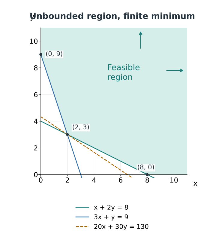
Both sloping inequalities exclude the origin. Shade their common allowed area in the first quadrant.

The lower boundary has three corners:

• On the y-axis, y >= 4 and y >= 9, giving (0, 9).
• The two sloping lines meet at (2, 3).
• On the x-axis, x >= 8 and x >= 3, giving (8, 0).

To verify the middle point, subtract x + 2y = 8 from twice 3x + y = 9. This gives 5x = 10, so x = 2 and y = 3.

Corner	C = 20x + 30y
(0, 9)	270
(2, 3)	130
(8, 0)	160

The smallest corner value is 130. Because the region is unbounded, add a check that no feasible point can give C < 130.

For this example, we can prove it directly:

14(x + 2y) >= 14(8) = 112
 2(3x + y) >=  2(9) = 18

Adding:
20x + 30y >= 130

Equality holds at (2, 3). Therefore, the minimum is 130 at (2, 3).

On a graph, the equivalent check is to draw 20x + 30y = 130 and examine the open half-plane 20x + 30y < 130. It has no overlap with the feasible region. The word “open” matters because the equality line contains our minimum point.

What if the question asks for a maximum instead?

Use the same region and objective. Points (t, 0) are feasible for every t >= 8.

At those points, C = 20t. You can keep increasing t, so there is no finite maximum. The largest entry in the corner table, 270, is not a maximum over the whole region.

An unbounded region describes the size of the allowed set. An unbounded objective describes the absence of a finite best value in the requested direction. These are different statements.

A minimum can fail too

Keep the same constraints, but minimise Z = 2x - y.

The corner values are -9, 1, and 16. It would be wrong to stop at -9.

Every point (0, t) with t >= 9 is feasible, and there Z = -t. As t increases, Z decreases without limit. This problem has no finite minimum.

These two changes of objective show why a corner table alone is insufficient for an unbounded feasible region.

The extra check for an unbounded region

After evaluating all its vertices, use the following test for the ordinary nonnegative-variable problems discussed here:

Required result	Candidate from corners	Check for a better feasible point
Maximum	Largest value M	Does ax + by > M overlap the region?
Minimum	Smallest value m	Does ax + by < m overlap the region?

If the better-value half-plane has no common point with the feasible region, the candidate is the optimum. This check is also described in the NCERT Exemplar’s linear programming exercises on IIT Kanpur’s SATHEE.

If there is overlap, the corner candidate is not an optimum. For these standard problems, the objective is unbounded in the requested direction. Show a feasible direction or a family of points, as we did above, to make the conclusion clear.

Do not close an open region along the top or right edge of your graph paper. Those edges are simply where you stopped drawing.

Worked example 3: when an entire edge is optimal

Return to the workshop’s original feasible polygon, but change the objective to:

Maximise Q = 40x + 40y

Since x + y <= 9, every feasible point has Q <= 360.

Both B (5, 4) and C (3, 6) reach 360. So does (4, 5), halfway between them.

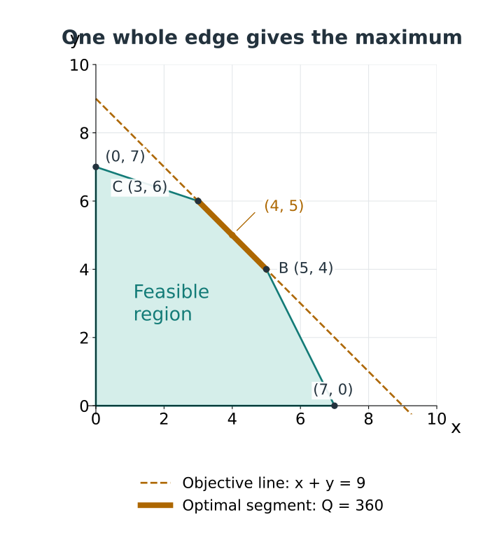
To find the complete optimal set, substitute y = 9 - x into the other two constraints:

2x + (9 - x) <= 14  gives x <= 5.
x + 3(9 - x) <= 21  gives x >= 3.

Therefore, the answer is:

Maximum Q = 360 at every point on x + y = 9 with 3 <= x <= 5.

Do not write “the whole line is optimal”. For example, (6, 3) lies on x + y = 9, but it requires 15 cutting slots and fails 2x + y <= 14.

Two equal values also need to be the best values before you conclude that their connecting segment is optimal. A tie between two nonoptimal corners proves no such thing.

What if there is no feasible region?

Suppose the conditions include:

x + y <= 4
x + y >= 7
x >= 0, y >= 0

No pair can have a sum at most 4 and at least 7. The two required half-planes have no common point.

The problem is infeasible, so there is no feasible solution to optimise. An objective value of zero is not the answer: even (0, 0) fails the second constraint.

This is different from an unbounded objective. In our unbounded examples, many allowed points existed; the objective simply kept improving without reaching a finite best value.

Three details that prevent avoidable mistakes

A redundant constraint may add no new edge

Add x + y <= 12 to the original workshop problem. The existing limit x + y <= 9 already guarantees it.

The extra condition changes neither the feasible region nor its corner points. You can check it, but you should not invent a new corner just because another line has been drawn.

An equality can reduce the region to a segment

If x + y = 5, together with x >= 0 and y >= 0, the feasible set is the segment from (5, 0) to (0, 5).

For Z = 2x + 3y, substituting y = 5 - x gives Z = 15 - x, where 0 <= x <= 5. The minimum is 10 at (5, 0) and the maximum is 15 at (0, 5). There is no two-dimensional area to shade.

Do not round a fractional solution without checking

Consider maximising Z = 3x + 2y subject to x + y <= 4.5, x <= 3, y <= 3, and nonnegativity.

For continuous variables, the optimum is (3, 1.5), with Z equal to 12. One check is Z = 2(x + y) + x <= 9 + 3 = 12.

Rounding to (3, 2) violates x + y <= 4.5. If the question requires whole numbers, integer x and y imply x + y <= 4. Then Z = 2(x + y) + x <= 8 + 3 = 11, attained at (3, 1).

The ordinary graphical solution and the whole-number solution answer different mathematical requirements. Read the wording before deciding which one is needed.

A clear order for your written solution

1. Define each variable and its unit.
2. State whether you are maximising or minimising, then write the objective.
3. List every constraint, including nonnegativity when required.
4. Draw and label the boundary lines using a clear scale.
5. Mark the common feasible region.
6. Find its vertices and check them against all constraints.
7. Calculate the objective at each valid vertex.
8. For an unbounded region, check whether better values remain possible.
9. State the optimum value and the corresponding variable values in words.

Before moving on, pause at step 6. This is where you catch infeasible intersections, missing axis corners, and plotting estimates that should have been exact fractions.

Try these six practice questions

Cover the answers and sketch the regions yourself. Each question targets a different decision.

1. Choose the correct side

For 2x - y >= 3, does the origin belong to the allowed region? Is the required side above or below the boundary?

Answer: The origin gives 0 >= 3, which is false. Rearranging gives y <= 2x - 3, so keep the side below the line, including the line itself.

2. Find every corner

Use x + y <= 6, x <= 4, y <= 5, and x, y >= 0. Maximise Z = 3x + 2y.

Answer: The corners are (0, 0), (4, 0), (4, 2), (1, 5), and (0, 5). Their values are 0, 12, 16, 13, and 10. The maximum is 16 at (4, 2).

3. Check a suspicious intersection

For x + y <= 7, 2x + y <= 10, x + 2y <= 11, and nonnegativity, is the intersection of x + y = 7 and 2x + y = 10 feasible?

Answer: The intersection is (3, 4). It gives x + 2y = 11, so it passes the third condition too. It is a valid corner where all three resource boundaries meet. Three lines crossing at one point still give only one point to test.

4. Find a minimum away from the origin

Minimise Z = 3x + 5y subject to x + y >= 5, x <= 6, y <= 4, and nonnegativity.

Answer: The corners are (5, 0), (6, 0), (6, 4), and (1, 4). Their values are 15, 18, 38, and 23. The region is bounded, so the minimum is 15 at (5, 0). The origin is infeasible.

5. Recognise multiple optimal points

Maximise Z = 6x + 3y subject to 2x + y <= 10 and x, y >= 0.

Answer: Since Z = 3(2x + y), the maximum is 30 along the entire segment from (5, 0) to (0, 10), including both endpoints.

6. Distinguish minimum from maximum

For x + y >= 6, x, y >= 0, consider Z = x + y.

Answer: The minimum is 6 along the segment from (6, 0) to (0, 6). There is no finite maximum: (t, 0) is feasible for every t >= 6, and Z equals t there.

Sources and further reading

The worked examples and diagrams in this guide use original numbers. These teaching resources support the underlying methods:

• OpenStax, Contemporary Mathematics, section 5.11: Linear Programming, for objectives, constraints, and graphical applications.
• OpenStax, Intermediate Algebra 2e, section 4.7: Graphing Systems of Linear Inequalities, for test points and shared solution regions.
• MIT OpenCourseWare, Geometry and Visualizations of Linear Programs, Spring 2013, especially slides 21 to 28, for boundedness, convexity, and corner-point conditions.
• James Jones, Richland College, Linear Programming: Table of Corner Points, updated June 2006, for filtering intersections and interpreting multiple optimal points.
• NCERT Exemplar, Linear Programming, hosted by IIT Kanpur’s SATHEE, for further work on unbounded-region checks and equal optimal values.

Frequently asked questions

1. What is the feasible region in linear programming?

It is the set of all points satisfying every constraint at the same time. For inequalities that include equality, the permitted boundary points belong to the region too.

2. How do I know which side of a line to shade?

Substitute a point that is not on the boundary into the original inequality. If the statement is true, keep that point’s side. If it is false, keep the opposite side.

3. Can I always use the origin as the test point?

No. If the boundary passes through the origin, it gives equality and does not identify a side. Choose another simple point off the line, such as (1, 0) or (0, 1) when suitable.

4. Is every intersection of two lines a corner point?

No. An intersection outside the common feasible region must be rejected. A valid vertex belongs to the region and satisfies all the constraints, including any bounds on individual variables.

5. Should I include corners on the coordinate axes?

Yes, when they are vertices of the feasible region. The conditions x >= 0 and y >= 0 can make the axes part of its boundary. The origin itself is included only if it satisfies every constraint.

6. Does an unbounded feasible region mean there is no answer?

No. Our minimisation example has an unbounded region but a minimum of 130 at (2, 3). You must examine the objective in the requested direction before deciding whether a finite optimum exists.

7. Why is checking just the corner table unsafe for an unbounded region?

The region continues beyond its vertices, and the objective may keep improving along that continuation. Check the relevant better-value half-plane or show algebraically that improvement is impossible.

8. What does it mean when two corners give the same optimum?

Every point on the segment joining those optimal corners also gives that value in the continuous problem. State the segment, including its endpoints. The full extended line need not be feasible.

9. Can the minimum occur at a point other than the origin?

Yes. The origin may be excluded by a minimum-requirement constraint, as in practice question 4. Even when it is feasible, the objective’s coefficients matter. Compare the actual feasible vertices and check boundedness.

10. What should I write if the shaded regions do not overlap?

State that the problem is infeasible because there is no point satisfying all the constraints. There is then no feasible solution to maximise or minimise.

11. Should I round fractional corner coordinates?

Keep exact fractions for the continuous problem. If whole numbers are explicitly required, check the feasible integer choices separately. Rounding may violate a constraint or miss a better allowed point.

12. Must an optimal point use every resource fully?

No. In the workshop example, the best plan uses all the packing and cutting capacity but leaves 4 finishing slots unused. Optimal means the best objective value among allowed choices, not complete use of every resource.