Price Elasticity of Demand: Which Method Should You Use?

A stationery shop reduces the price of a notebook. More students buy it, but has the shop collected more money? And how strongly did purchases respond to the lower price?

Those are related questions, but they do not ask for exactly the same answer. One needs a calculation of responsiveness. Another needs a comparison of total spending. A third question might give you only a point on a demand curve.

That is why price elasticity of demand has several measurement methods. The trick is to read the information before reaching for a formula.

This guide takes you through the percentage method, total expenditure method, and geometric method, using original examples you can solve alongside the explanation. We will also deal with the awkward moment when two apparently sensible calculations give different numbers.

Choose Your Method in 30 Seconds

What the question gives you	Best starting point	What you can find
Percentage changes in price and quantity	Percentage method	A numerical elasticity
Original and new prices and quantities	Percentage method using the stated base	A numerical elasticity
Two observations with an instruction to use averages	Midpoint or arc method	Elasticity across the interval
Price and total spending before and after a change	Total expenditure method	Elastic, inelastic, or unit elastic
A point on a straight demand line with axis intercepts	Geometric method	Point elasticity
A demand equation and a specified price	Find quantity and the rate of change	Point elasticity

If the question names a method, use it. If it asks for an exact coefficient, a statement such as “elastic” is incomplete. If it asks only for the degree of elasticity using expenditure, you do not need to invent an exact coefficient.

First, Decide What Your Elasticity Number Means

Price elasticity of demand measures how responsive quantity demanded is to a change in the good’s own price, with other influences held constant.

We will use E for its positive magnitude. Thus, E = 2 means the percentage response of quantity is twice the percentage price change under the measurement being used.

• E > 1: elastic demand.
• E = 1: unit elastic demand.
• 0 < E < 1: inelastic demand.
• E = 0: perfectly inelastic demand.
• E tends to infinity: perfectly elastic demand in the limiting case.

For an ordinary downward-sloping demand curve, the signed ratio is negative because price and quantity move in opposite directions. A signed answer of -2 and a magnitude of 2 describe the same responsiveness. State your convention instead of treating the minus sign as a mistake. OpenStax: Price Elasticity of Demand

These calculations concern a movement along a demand curve. If a festival, advertising campaign, or income change also affects purchases, the before-and-after sales figures alone cannot isolate the effect of price. Revise movement along a demand curve versus a shift if that distinction feels uncertain.

Method 1: Percentage or Proportionate Method

The basic calculation is:

E = |Percentage change in quantity demanded / Percentage change in price|

The vertical bars mean “take the magnitude”. You can retain signs in your working and make the final classification from the magnitude.

When the question uses original values as the base:

Percentage quantity change = (Q2 - Q1) / Q1 × 100

Percentage price change = (P2 - P1) / P1 × 100

Combining the two gives:

E = |[(Q2 - Q1) / (P2 - P1)] × (P1 / Q1)|

Here, P1 and Q1 are the original price and quantity; P2 and Q2 are the new values. The 100s cancel. That is why the shorter formula has no extra multiplication by 100 at the end.

Worked Example 1: A Notebook Price Cut

A shop cuts the notebook price from Rs 60 to Rs 54. Weekly quantity demanded rises from 200 to 250 notebooks. Use original values as the base.

Step 1: Find the changes.

Price change = 54 - 60 = -Rs 6.

Quantity change = 250 - 200 = 50 notebooks.

Step 2: Turn both into percentages.

Percentage price change = (-6 / 60) × 100 = -10%.

Percentage quantity change = (50 / 200) × 100 = 25%.

Step 3: Divide and interpret.

E = |25 / -10| = 2.5.

Demand is elastic under this calculation. The 10% price reduction is associated with a 25% increase in quantity demanded.

A clear final answer would be: “The magnitude of price elasticity of demand is 2.5. Demand is elastic because the proportionate quantity response exceeds the proportionate price change.”

Worked Example 2: Find the Missing Quantity

At Rs 80 per bottle, quantity demanded is 150 bottles. Price rises by 10%. The magnitude of elasticity is 0.6, measured using original-value percentages. Find the new quantity demanded.

Percentage fall in quantity = 0.6 × 10% = 6%.

Fall in quantity = 6% of 150 = 9 bottles.

New quantity demanded = 150 - 9 = 141 bottles.

The new price is Rs 88. You can check the answer by dividing the 6% quantity fall by the 10% price rise.

Notice the direction. The formula supplies a magnitude, but the demand relationship tells you whether to add or subtract the quantity change.

When Only Percentages Are Given

Suppose quantity demanded falls by 18% after price rises by 12%.

E = 18 / 12 = 1.5, so demand is elastic.

Do not divide the new quantity by the new price. Elasticity compares changes relative to their bases, not the levels of price and quantity themselves.

Why the Midpoint Method Can Give a Different Answer

Return to the notebook example: price moves from Rs 60 to Rs 54, and quantity moves from 200 to 250.

The original-base answer was 2.5. If you reverse the journey and use 54 and 250 as the starting values, the percentage bases change. Your answer becomes 1.8.

Nothing mysterious happened to the observations. You changed the denominators.

The midpoint method uses the same average price and average quantity in either direction:

Average price = (P1 + P2) / 2

Average quantity = (Q1 + Q2) / 2

E = |[(Q2 - Q1) / average quantity] / [(P2 - P1) / average price]|

For our notebooks:

• Average price = (60 + 54) / 2 = Rs 57.
• Average quantity = (200 + 250) / 2 = 225 notebooks.
• E = |(50 / 225) / (-6 / 57)| = 19/9, or approximately 2.11.

The midpoint answer measures responsiveness across the interval using average bases. Reversing the two observations leaves its magnitude unchanged. It need not equal an original-base calculation. OpenStax: Midpoint Method

Method 2: Total Expenditure or Total Outlay Method

Calculate how much buyers spend before and after the price change:

Total expenditure = Price × Quantity purchased

For the same transactions, this is also the seller’s total revenue. We assume the quantities in the exercise are actually bought and sold.

Then compare the direction of the price change with the direction of the expenditure change:

Price change	Expenditure change	Classification
Rises	Falls	Elastic
Falls	Rises	Elastic
Rises	Rises	Inelastic
Falls	Falls	Inelastic
Changes	Stays the same	Unit elastic

For a finite pair of observations on an ordinary downward demand relationship, these classifications agree with the midpoint elasticity. A point-elasticity interpretation describes small changes near that point. Keeping the distinction in mind avoids conflicts with original-base percentages.

The expenditure test tells you which side of one the elasticity lies. By itself, a rise in spending after a price cut does not establish whether E is 1.4 or 3.2. OpenStax: Elasticity and Pricing

Worked Example 3: Three Different Customer Responses

Three hypothetical stalls each begin with a price of Rs 50 and sales of 100 units. Each reduces price to Rs 40.

Initial expenditure at every stall = 50 × 100 = Rs 5,000.

Stall	New quantity	New expenditure	Result
A	140	40 × 140 = Rs 5,600	Elastic
B	110	40 × 110 = Rs 4,400	Inelastic
C	125	40 × 125 = Rs 5,000	Unit elastic

At stall A, buyers purchase enough extra units to more than offset the lower price. Spending rises.

At stall B, purchases increase, but only slightly. The extra sales do not compensate for receiving Rs 10 less per unit.

At stall C, the two effects exactly balance in money terms. The price reduction from 50 to 40 requires quantity to rise from 100 to 125 to preserve expenditure.

A useful way to check stall C is old expenditure / new price = 5,000 / 40 = 125 units.

Worked Example 4: Quantity Is Not Given

A product’s price rises from Rs 30 to Rs 36. Total spending falls from Rs 3,000 to Rs 2,880. Classify elasticity using expenditure.

Price rises while expenditure falls, so demand is elastic over the interval.

That completes the requested method. If you want to verify the underlying quantities, they were 3,000 / 30 = 100 units and 2,880 / 36 = 80 units. The midpoint coefficient is 11/9, approximately 1.22, which confirms the classification.

Do not call demand unit elastic just because both changes have an absolute numerical value that looks similar. Rupees of price, units of quantity, and rupees of total expenditure are different measurements.

The Equal-Percentage Trap

Here is a small calculation that saves a lot of confusion.

Suppose price rises by 20% and quantity falls by 20%, both measured from their original values. Does spending remain unchanged?

Start with price Rs 100 and quantity 100. Spending is Rs 10,000.

After the changes, price is Rs 120 and quantity is 80. Spending becomes Rs 9,600.

It falls by 4%. Multiplying 1.20 by 0.80 gives 0.96, not 1.

The original-base elasticity is 1, but the midpoint elasticity is 11/9, greater than 1. The expenditure test agrees with the midpoint result.

To maintain spending after a 20% price rise, quantity must become 100 / 1.20 = 83.33 units, approximately. That is a fall of 16.67%, rather than 20%.

The familiar unit-elastic rule is exact for a constant-expenditure demand relationship, and point elasticity gives the local result for very small changes. Equal and opposite finite original-base percentages do not exactly cancel. NCERT’s mathematical discussion explicitly identifies the extra product-of-changes term that is ignored in the small-change approximation. NCERT: Theory of Consumer Behaviour, expenditure discussion

Method 3: Geometric or Point Method

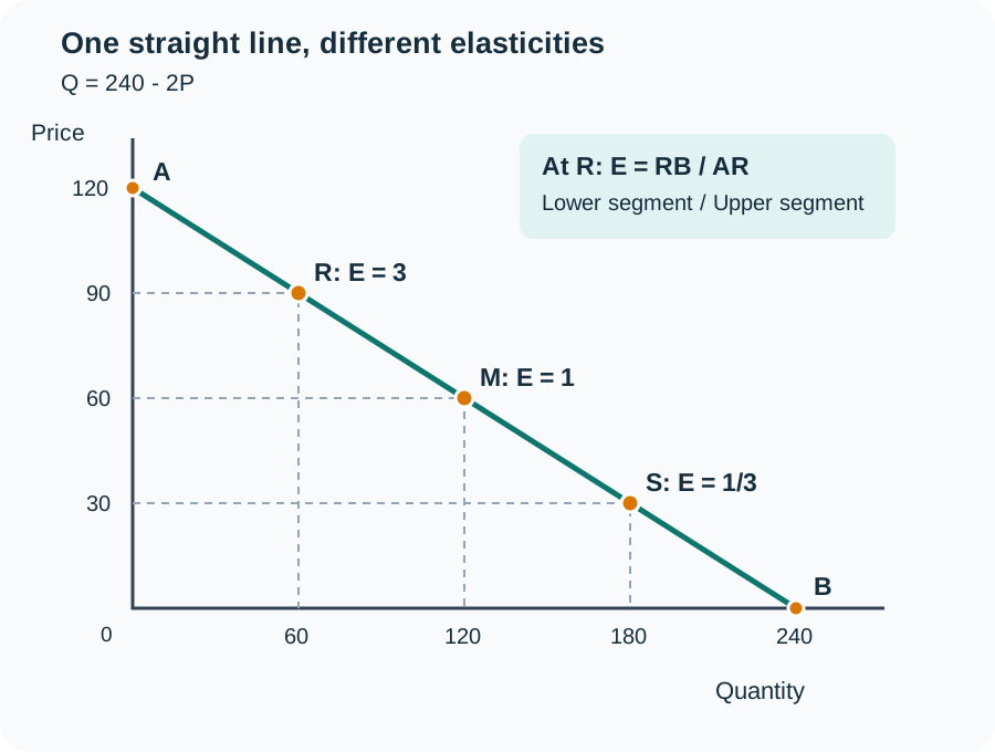
Draw a downward-sloping straight demand line. Label its price-axis intercept A and quantity-axis intercept B. Choose a point R on the line.

E at R = RB / AR = Lower segment / Upper segment

RB is the segment from R down to the quantity axis. AR is the segment from the price axis down to R. Measure both along the same demand line, using the same unit.

The ratio describes elasticity at R, not an average for the entire line. This geometric rule for linear demand is explained in NCERT’s consumer behaviour chapter.

Worked Example 5: Read the Segments

Suppose AR measures 2 cm and RB measures 6 cm on a correctly drawn demand line.

E = RB / AR = 6 / 2 = 3.

Demand is elastic at R.

If you accidentally use AR / RB, you obtain 1/3 and reverse the classification. Label the lower segment before you divide.

You may use supplied segment lengths. Do not measure an unscaled sketch with a ruler and assume it contains accurate numerical information.

Worked Example 6: Use an Equation to Check the Diagram

For our diagram, the demand equation is:

Q = 240 - 2P

At P = 90, Q = 240 - 180 = 60.

Each Rs 1 increase in price reduces quantity by 2 units along this line. Its point elasticity magnitude is therefore:

E = 2 × P / Q

At R: E = 2 × 90 / 60 = 3.

At M, P = 60 and Q = 120. E = 2 × 60 / 120 = 1.

At S, P = 30 and Q = 180. E = 2 × 30 / 180 = 1/3.

The demand line has the same slope throughout, but elasticity changes because P/Q changes. A rupee means a different percentage of Rs 90 than of Rs 30; ten units mean a different percentage of 60 than of 180.

For a differentiable demand equation, the general point formula is E = |dQ/dP| × P/Q. For a straight line Q = a - bP, this becomes E = bP/Q. The distinction between point and arc calculations is also set out in the University of Victoria demand and supply notes.

What Happens Across the Whole Line?

For a downward straight line meeting both positive axes:

• In its upper half, the lower segment is longer: E > 1.
• At its midpoint, the two segments match: E = 1.
• In its lower half, the lower segment is shorter: E < 1.
• Approaching the price-axis intercept, quantity tends to zero and elasticity tends to infinity.
• Approaching the quantity-axis intercept, price tends to zero and elasticity tends to zero.

Treat the endpoint labels as limiting values. The ordinary percentage calculation at zero quantity or zero price involves a zero base.

A straight demand line is therefore not unit elastic everywhere. A constant-expenditure curve such as PQ = 7,200, or Q = 7,200/P for positive P, is a rectangular hyperbola and has unit point elasticity throughout.

What If the Demand Curve Is Curved?

Do not divide the lengths of two curved portions. At a smooth interior point, point elasticity depends on the curve’s slope there. If a tangent at that point meets the positive price and quantity axes, apply the segment ratio to that straight tangent.

For the basic geometric problems in this guide, the demand line itself is straight, so no tangent construction is needed.

Connect All Three Methods Without Mixing Them

Use our line Q = 240 - 2P again. Move from P = 90, Q = 60 to P = 80, Q = 80.

Original-base percentage calculation:

E = |(20 / 60) / (-10 / 90)| = 3.

Midpoint calculation:

E = |(20 / 70) / (-10 / 85)| = 17/7, approximately 2.43.

Expenditure test:

Spending rises from 90 × 60 = Rs 5,400 to 80 × 80 = Rs 6,400, while price falls. The interval is elastic.

Geometric calculation at the starting point:

E = RB / AR = 3.

There is no contradiction. The original-base calculation matches starting-point elasticity here because the demand relationship is linear. The midpoint calculation describes the interval using average values. The expenditure test agrees on the interval’s classification without supplying its exact coefficient.

The numerical equality between the first and fourth answers is not a general rule for large movements on curved demand functions.

Common Mistakes and Quick Repairs

Mistake	Repair
Using change in quantity divided by change in price alone	Include the price-to-quantity factor or calculate both percentages
Mixing original and average bases	Write the method beside the formula
Calling -2 inelastic because it is below 1	Classify using magnitude, which is 2
Using upper segment divided by lower segment	Start at the point and identify the segment toward the quantity axis
Assuming a straight line has constant elasticity	Check P/Q at different points
Claiming the expenditure test gives an exact coefficient	State only the classification unless you do another calculation
Assuming more revenue means more profit	Check costs before drawing a profit conclusion

For example, a shop may collect Rs 1,000 more after a discount but spend Rs 1,300 more on the extra units sold. Revenue rises while profit falls. Elasticity helps analyse receipts; it does not remove the need to consider costs.

Try These Eight Questions

Use the method stated. Keep exact fractions until the final step where possible.

1. Price falls by 8% and quantity demanded rises by 12%. Find E using these percentages.
2. Price rises from Rs 40 to Rs 44. Quantity falls from 300 to 285. Use original bases.
3. Price falls from Rs 25 to Rs 20. Spending rises from Rs 2,000 to Rs 2,200. Use expenditure.
4. Price falls from Rs 80 to Rs 64. Initial quantity is 50. Find the new quantity needed to keep expenditure unchanged.
5. On a demand line, the upper segment is 9 cm and the lower segment is 3 cm. Find point elasticity.
6. For Q = 180 - 3P, find point elasticity at P = 40.
7. Price falls from Rs 30 to Rs 20 and quantity rises from 40 to 60. Find midpoint elasticity.
8. A 10% price rise accompanies a 10% quantity fall, using original bases. By what percentage does expenditure change?

Answers With Working

1. E = 12 / 8 = 1.5, elastic.

2. Price rises by 4/40 × 100 = 10%. Quantity falls by 15/300 × 100 = 5%. E = 0.5, inelastic.

3. Price falls and expenditure rises, so demand is elastic over the interval.

4. Old expenditure = 80 × 50 = Rs 4,000. New quantity = 4,000 / 64 = 62.5 units, assuming the good is divisible.

5. E = 3 / 9 = 1/3, inelastic at the point.

6. Q = 180 - 3 × 40 = 60. E = 3 × 40 / 60 = 2, elastic.

7. Average price = 25; average quantity = 50. E = |(20/50) / (-10/25)| = 1. Both observations also give expenditure of Rs 1,200.

8. New spending is 1.10 × 0.90 = 0.99 of old spending. It falls by 1%.

A Short Checklist Before You Submit

Underline the requested method. Identify whether the question concerns a point or an interval. Label the price and quantity values, keep percentage bases consistent, and state whether you are reporting a signed coefficient or its magnitude.

Then add a sentence explaining your answer. “E = 0.5, so demand is inelastic” is more useful than a bare number. For an expenditure question, name both directions: “Price rises and expenditure falls, so demand is elastic.”

If you want to revise the wider idea before another practice round, read our introduction to elasticity of demand.

Frequently Asked Questions

Which method should I use when the question gives two prices and two quantities?

Follow any named method first. Use original values when the question specifies original-base percentages; use averages when it asks for midpoint or arc elasticity. If neither is specified, state your convention clearly and follow the approach expected in your exercise.

Are the percentage and proportionate methods different?

They express the same idea. Dividing the proportionate quantity change by the proportionate price change gives the same answer as dividing their percentage changes because the two factors of 100 cancel.

Why is price elasticity of demand usually negative?

On an ordinary downward-sloping demand curve, price and quantity move in opposite directions. The signed ratio is negative. Elastic, unit elastic, and inelastic classifications usually use its positive magnitude.

Can the expenditure method calculate an exact elasticity of 2?

Not from the direction of expenditure alone. It can establish that demand is elastic, meaning the relevant magnitude exceeds 1. To obtain an exact coefficient, use the price and quantity information with a numerical method.

What is the easiest way to remember the expenditure test?

Compare price with total spending. Opposite directions indicate elastic demand; the same direction indicates inelastic demand. Unchanged spending with a price change indicates unit elasticity over the interval under the midpoint measure.

Is geometric elasticity upper segment divided by lower segment?

No. It is lower segment divided by upper segment. With A on the price axis, B on the quantity axis, and R between them, use RB/AR.

Does a straight demand curve have the same elasticity everywhere?

No. Its slope is constant, but its price-to-quantity ratio varies. Elasticity falls as you move down a straight demand line from the price axis toward the quantity axis.

Is demand unit elastic at every point on a rectangular hyperbola?

Yes, when the curve represents a positive constant expenditure relationship, PQ = k. Its point elasticity magnitude is 1 throughout, and spending remains k at every point.

Why can an original-base answer disagree with the expenditure test?

Finite original-base percentages use starting values, while the expenditure test for two observations agrees with midpoint elasticity. The difference matters near unit elasticity or for large changes. Check the method and calculate the actual price-times-quantity totals.

Does elastic demand mean a price cut always increases profit?

No. A price cut over an elastic interval raises total revenue under the stated demand assumptions. Profit also depends on the cost of supplying the extra units, so you need cost information before concluding that profit rises.